Sample Video Clips of Animation Results Using FastBEM Acoustics®:
- Modeling of a sound barrier (at ka = 393, length of the barrier = 78.5 m)
- Sound wave from a point source interacting with a perforated plate (at ka = 150)
- Sound wave from a point source interacting with a perforated plate (at ka = 30)
- A speaker model with radiated sound waves (at ka = 10)
- A sphere interacting with two plane waves in the +x and +y directions (at ka = 2)
- A sphere interacting with a plane wave traveling in the -x direction (at ka = 2)
- Sound waves radiated from a pulsating sphere (at ka = 2)
Application Examples:
Several application examples are presented below to demonstrate the capabilities of the FastBEM Acoustics® software in solving large-scale acoustic problems (For other examples, check out the Home page or the videos listed above. For verification examples, visit the Verification Cases page). All the examples are solved on a laptop PC with an Intel® Core i7-13800H CPU and on Windows® 11 OS. The tolerance for convergence is set at 1.E-4 in all cases (To view larger and better-quality plots or videos, click on the images).
A. Wind Turbine Model
This is a half-space acoustic BEM model used to predict the wind turbine noise. In this example, five wind turbines are modeled with 557,470 boundary elements. All the turbines have a height of about 29 m and are spaced 50 m apart in the x- and y-directions. The ground is modeled as a rigid infinite plane where no elements are applied because of the use of the half-space Green's function in the code. The sound pressure on the surfaces of the turbines and a field surface of the size 200x200 m^2 on the ground are computed using the FastBEM Acoustics® software at ka = 5 (representing a rotating speed of 3 cycles/s for the blades). This model was solved in 4 min. The sound pressure on the surfaces of the turbines and the field surface (the ground) are shown in the following Video.
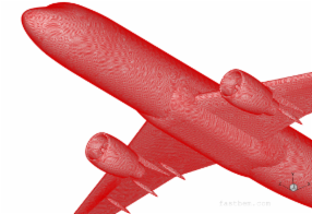
B. Airbus A320 Model
The noise during the landing of an airplane is simulated using a BEM model of the Airbus A320 airplane. There are 539,722 elements for this BEM model. The acoustic pressure fields on the surface of the airplane due to the vibrations of the two jet engines and on the ground are computed using the FastBEM Acoustics® software at ka = 61.5 or f = 90 Hz. The BEM model was solved in 25 min. using the PC. The mesh plot and the sound pressure plot are shown below (Click on the animation to watch the video).

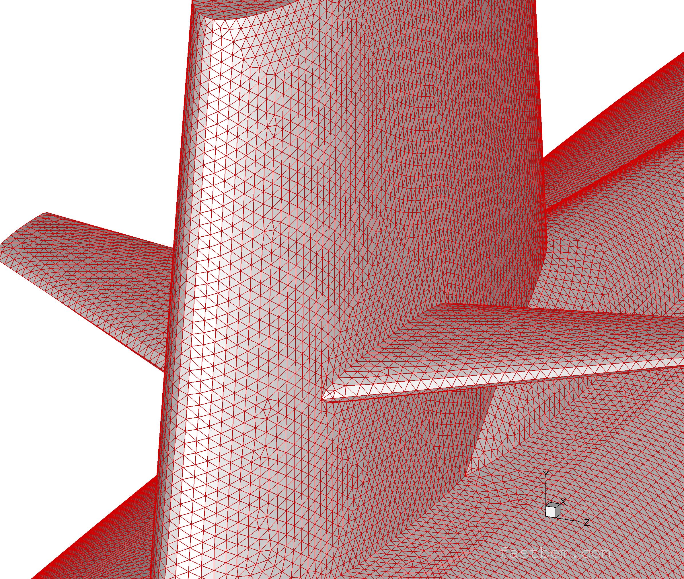
C. Skipjack Submarine Model
There are 250,220 DOFs in this model of the Skipjack submarine immersed in water in a half space. The sound pressure on the surface of the submarine due to the rotation of the propeller and an incident wave in the (1, 0, -1) direction at ka = 383.7 (f = 1233 Hz) is computed using the FastBEM Acoustics® software. The model was solved in 7 min. on the PC. The first figure below shows the boundary element mesh used and the second shows the plot of the acoustic pressure on the surface of the structure. The video shows the sound pressure radiated onto the sea floor from the submarine without the incident wave.

D. Street Block Model
A street block is modeled here to study the propagation of sound waves from different sources and their interacting with the buildings. The mesh has 273,870 elements on the buildings and a large field surface placed on the ground to calculate the sound waves. The following two videos show the sound fields due to a plane incident wave along the x-direction and three point sources along the main street, respectively, at the frequency f = 200 Hz or ka = 366. The interactions of the sound waves with the buildings are observed from these simulations. The BEM models were solved in 4 min. on the PC.
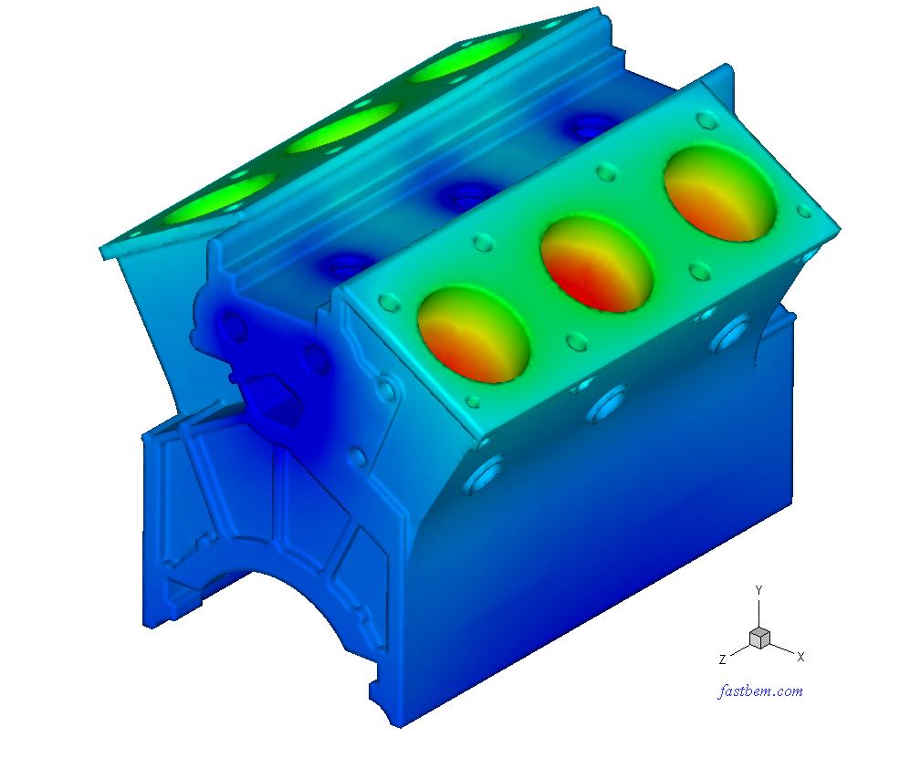
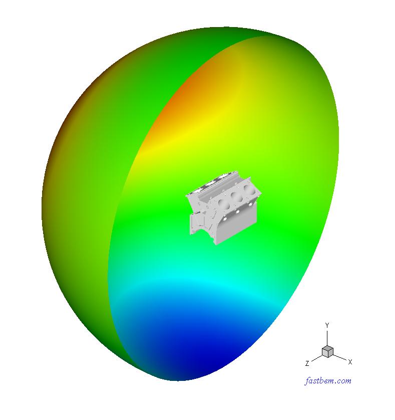
E. Engine Block Model
An engine block is modeled with 132,764 boundary elements. The largest dimension of the engine model is 360 mm. Velocity boundary conditions are applied to the surface of the engine block. The acoustic pressure on the surfaces of the engine block and a field surface surrounding the engine are computed at ka = 3.6 (f = 546 Hz). The model was solved in less than 2 min. using the PC. The plots of the acoustic pressure on the surface of the engine block and the field surface are shown below.